Keywords: Hydrogeology, Artificial Neural Networks (ANN),Machine Learning (ML).

Abstract

The knowledge of hydrogeological system functionality, is of vital importance for its management and sustainable development. One of the variables and main input it feeds this system is the recharge (R) product of precipitation (P). The purpose of this study is a non-linear regressor model using artificial neural networks (ANN). For the above, with INETER data collected, it was estimated R using input variables for instance: precipitation (P), soil textures, and other known environmental variables in Managua Aquifer. With the information collected, data exploration or ‘Data mining’ was carried out through descriptive statistics, which allows for presenting, interpreting, and analyzing the data comprehensively. Using the Python programming language (Rossum, 1991) and the JupyterLab work environment, the ANN elements were developed through the Scikit-Learn library or better known as Sklearn (Cournapeau, 2010). After the iterations and settings of hyperparameters, a better fit will be improved using the cost function, which determines the error between the estimated value and the observed value, to optimize the parameters of ANN. In the end, the final configurations of ANN are indicated for each soil texture.

1. Introduction

Advances in computer modeling, computing power, and information processing have resulted in improved and practical tools for better understanding highly complex natural systems. A great deal of work has been focused on the applicability of Machine Learning (ML) methods in hydrology (Shortridge J.E, 2019) and hydrogeology (Tao et al, 2022) science. However, no single technique is used, as the data and scenario available will determine the most appropriate method for a given problem. (S. et al, 2017). Approaches based on ML and hydrological modeling are important areas of research. These models are more suitable for water resource studies than physical models. (Kenda K & Klemen, 2019) The most common method for the prediction of groundwater resources using Machine Learning (ML) techniques is the Artificial Neural Network (ANN). ML methods use hidden patterns in historical data and then apply these patterns to predict future scenarios. (S. et al, 2017)

In Nicaragua the main source of the drinking water supply comes from groundwater and it represents 70% of the supply, (FAO, 2013), but this source is one of the little-studied sources in Nicaragua and Central America; for this reason, new research technologies have been developed over the years that promote management of water resources helping to improve access to water for the population. In recent years studies have been developed focused on groundwater recharge estimate (INETER, 2020) and in detail the hydrogeological characteristics of the Las Sierras aquifer (INETER, 2020) to obtain approximate data on the groundwater recharge.

The importance of this document is the design of a nonlinear regressor model of Machine Learning (ML) that estimates or simulates Potential Recharge (PR), based on historical precipitation data, field information, geological survey, and infiltration tests. In this regard, there is no national bibliography dedicated to the use of ML in hydrology and hydrogeology. Initially, it is intended to prepare the ANN using the input data, generation of the hidden layers, and outputs. Subsequently, the ‘backpropagation’ will be carried out, which is the training section of the network using the training set. Finally, the configuration is obtained, which will provide the estimated outputs with the least error concerning the observed or test data.

2. Materials y Methods

2.1. Study area

Las Sierra’s aquifer (568.51 Km2) is located in the city of Managua covering the municipalities of Ticuantepe, Masaya, La Concepción, El Crucero, San Marcos, Nindirí, Managua, Ciudad Sandino, and Tipitapa. (Figure 1) In geomorphological theme, it is located on the central-western edge of a regional structure called the Nicaraguan Depression compound predominantly with tertiary and quaternary volcanic lithological material (INETER, Mapa de las Provincias Geológicas de Nicaragua, 2004).

Based on the modified Köppen methodology (Köppen, 1918), there is a dominant climatic subtype category: Awo (w) igw, Warm Sub-humid with less humidity, with a heat wave period (canicula). According to the 1971 -2010 meteorological historical record, Managua shows a well-defined rainy season from May to October. During the period, there are 2 precipitation maximums, in June with 164.87 mm and in September with a monthly average of 220.53 mm. In November, the dry period is presented, where it is observed that rainfall decreases significantly with values from 53.45 mm in November to 2.93 mm in February, this being the driest month. Temperature behavior oscillates between the maximum value of 29.04ºC in April and the minimum value of 25.96ºC in December; values that have occurred in the dry period. From June (27.09°C), decreasing, lasting until December (25.96°C). This decrease in temperature coincides with the winter season of the countries located in the Northern Hemisphere and with the incursions of cold air masses of polar origin. (INETER, Atlas Climáticos. Periodo 1971 - 2010, 2022)

Hydrogeologically, this aquifer is considered unconfined, although localized semi-confined conditions have been recorded due to the presence of silt-clay thin layers and lava flows with low fracturing. (Losilla y otros, 2001) The main geological units are La Sierra formation (TpQs) and the quaternary alluvial materials (Qal). (INAA/JICA, 1993) Natural groundwater recharge is caused by rainwater that infiltrates into the aquifer. Since precipitation is directly proportional to elevation, it is generally considered that it increases with the same trend, greater in the high zone (south) and less in the low zone (north). However, recent studies indicate that there is also recharge at intermediate levels, this also depends on the infiltration coefficient from the geological units, soil textures, and land use. (Losilla y otros, 2001).

The origin of the soil is volcanic and the soil textures that predominate in the area are sandy loam, clay loam, sand, and the waterproofed area as a result of urban development. (INETER, 2021)

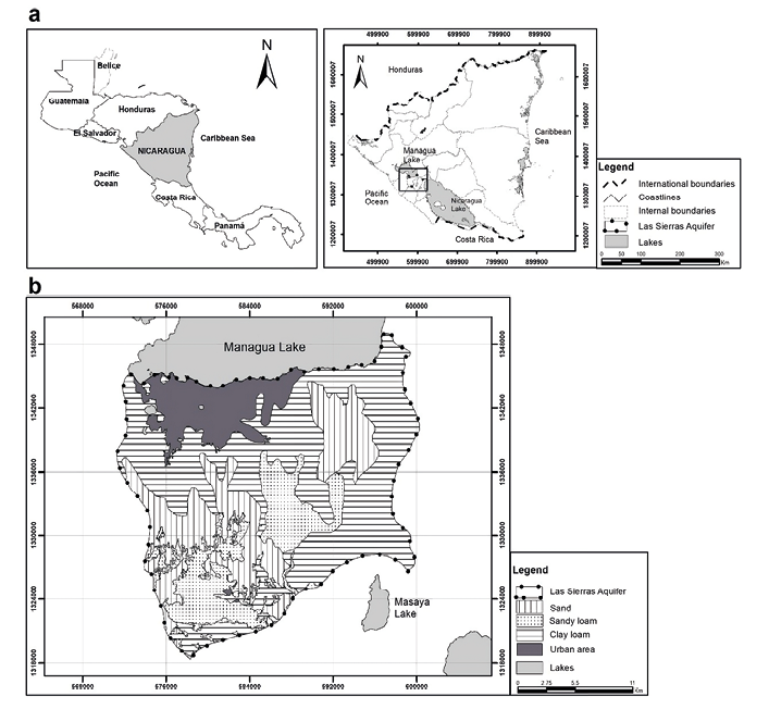
Figure 1 a: Aquifer Location, b: Soil texture. Source: self-made

2.2. Data

The selection of input variables is crucial for the development of data-driven models and is particularly relevant in water resource modeling. (Quilty et al, 2016) (Galelli et al, 62, 33–51). The database is made up of 576 observations and 33 variables (M>N), giving a total of 19,000 data. The origin of the variables is mainly the observations of INETER. The variables are categorized into 3 groups:

•Time: Includes observations record from 2005 to 2020 (15 years), with a monthly resolution.

•Soil characteristics: infiltration capacity, field capacity, wilting point, soil density, slope, type of vegetation, and root depth.

•Environmental variables: precipitation, air temperature, infiltrated precipitation, surface runoff, PE (potential evapotranspiration), soil moisture, and groundwater recharge (Gr).

According to the conceptual model, in the study area, there are 03 soil textures (INETER, 2021), which are associated with different infiltration and Gr values, therefore, the data has been divided into 03 groups: S01, S02, and S03 which correspond to the texture of sandy soil, sandy loam, clay loam respectively. An ANN was made for each soil texture. Regarding the variables of precipitation, temperature, and PE, monthly data from the stations ‘Airport’, ‘Salvador Allende’, ‘INETER’, and ‘Casa Colorada’ were used. For the estimation of PE and Gr was used Thornthwaite (Thornthwaite, 1948) and soil water balance (Schosinsky & Losilla, 2006) methods respectively.

2.3. ANN Desing

The Artificial Neural Network (ANN)

An Artificial Neural Network (ANN) is a distributed information processing system, where learning is based on neural processes. An ANN learns, memorizes, and reports the various relationships found in the data. The elementary unit of ANNs is the Artificial Neuron (AN), which is a simplified mathematical abstraction of the behavior of a Biological Neuron (BN). (Corea, 2014) ANNs are composed of several ANs grouped in layers and connected to solve a problem.

In Figure 2(b) it is the NA, which is similar to a dendrite tree of the BN, the AN receives a set of signals through the inputs x1, xi, xn. Each input is amplified or reduced by its corresponding weight value w1j, wij, wnj similar to the biological synapse), in such a way that the product of the binomial “input” times “weight” (xn * wnj) is added together with the threshold value called bias (bj) which is multiplied by the bias weight (wb). This product is transferred to the activation function “f “, which corresponds symbolically to the kernel of the BN. This function processes and generates the output of the NA (Reed & Marks, 1999) (Cortez et al, 2002). Equation 1 represents the mathematical model of the ANN.

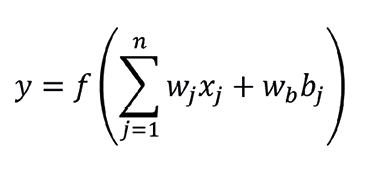
Equation 1: ANN Mathematical model

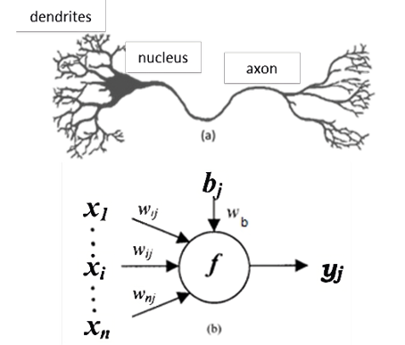
Figure 2: Representation of BN and AN. Source: Adapted from Reed & Marks, 1998 and ASCE, 2000.

Activation Function (AF)

The activation function (AF) controls the information that propagates from one layer to the next (forward propagation). The main goal of AF is to add non-linear components to the network, so an ANN without AF is very limited in predicting. The AF converts the net input value to the neuron (sum of weights and bias) into a new value (y). It is thanks to combining activation functions with multiple layers that ANN models can learn non-linear relationships.

In this study, the ReLu function (Rectified Linear Unit) was used. The use of this function goes back several decades, but it was not until 2010 (Glorot et al, 2010) that it was shown to be much better in most cases than other AFs in use at the time. The reason for this is a very low computational cost and the behavior of its derivative (gradient) is very simple: zero (0) for negative values and one (1) for positive values. ReLu is unbounded for positive numbers (Figure 3), which gives a constant gradient, leading to faster learning.

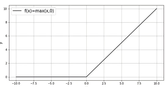
Figure 3: Activation function ReLu. Source: self-made

Preprocessed

This step consists of data treatment before the calculation. It should be noted that the ANN will be trained and tested with 80% and 20% data respectively, which represent approximately 12 and 3 years. The preprocessing consists of normalizing the training data. This process is necessary for the convergence of the ANN models and to improve their performance (Corea, 2014). The predictors are numeric and were normalized. All these processes were carried out with the ‘StandardScaler’ package from the ‘Sklearn’ library. This package subtracts from each value of an attribute the mean value of the column in which it is found (centered) and finally divides each predictor by its standard deviation (normalized), in this way the data have a normal distribution.

Hyperparameters

The hyperparameters of a model are the configuration values used during the training process. These are values that are not usually obtained from the data, so they are usually indicated by the data scientist. The optimal value of a hyperparameter cannot be known before a given problem so, random initial values have to be used which are adjusted by trial and error. In ANN the hyperparameters are the number and size of hidden layers, the learning rate, and alpha or the penalty parameter. When training a Machine Learning (ML) model the values of the hyperparameters are fixed, so that with these the weights (w) are adjusted generating the prediction values with the least error in contrast to the test data. For this study was initially considered as one (01) hidden layer with 10 neurons, 10 alpha values ranging between 10-3 and 103, and finally a learning rate of 10-2 and 10-1.

Regarding the hidden layer, the more neurons and layers, the greater the complexity of the relationships that the model can learn so, the number of parameters to learn increases and with it the training time. The number of neurons in hidden layers has a meaning in the action of the ANN; with few neurons, the network will approximate poorly while many neurons will overfit the training data. (ASCE, 2000).

In the case of the learning rate, if it is very high, the optimization process can jump from one region to another without the model being able to learn; on the contrary, if the learning rate is very little, the training process may take too long and not be completed. The objective of Alpha is to prevent the weights from taking excessively high values, thus preventing a few neurons from dominating the behavior of the network. This hyperparameter gets a ‘smooth’ model in which the outputs change more slowly when the inputs change.

Predictive model

To determine a better ANN configuration, the MLP or Multi-Layer Perceptron model was used through the ‘MLPRegressor’ package for regression analysis. The MLP is considered a universal approximator (Hornik et al, 1989), and has been used successfully in hydrological modeling. (ASCE, 2000) (Maier & G. C., 2000). This package consists of a “solver” and “interactions value”. The solver is used for the optimization of the weights (w). In this case, the ‘lbfgs’ was used, which is an optimizer of the Quasi-Newton family of methods and is used for a few data (observations <1000), allowing a faster and better conversion. Finally, the ANN has been instructed to work with a maximum of 1000 iterations. The design process of the ANN is described in the process diagram of Figure 4.

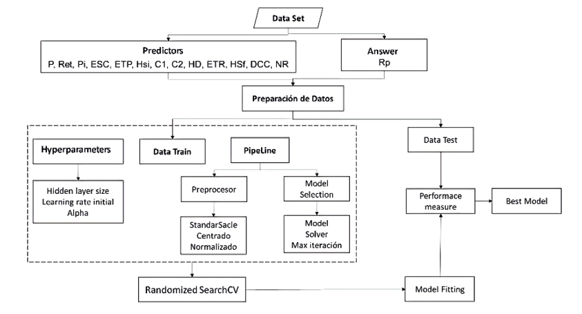
Figure 4: ANN Process Diagram. Source: self-made

ANN Training

This is similar to the idea of calibration, which is an integral part of hydrological modeling studies. The purpose of the training is to determine the set of connection weights and nodal thresholds so that the ANN estimates outputs close enough to the observed values. To do this, the gradient descent algorithm, ‘backprogation’, and the cost function are used. Using the cross-validation algorithm or “randomizedsearchCV”, the training set is divided into folders (50 in this case) which are evaluated in the ANN and their final result (prediction) is contrasted with the output data (observed) using a cost function.

The target is to reduce the error; therefore, the descent gradient is used to estimate the vector gradient associated with the adjustment parameters (weights and bias). This vector is added to the learning rate and then subtracted from each weight (w). To update or adjust the weights (w) the ‘backprogation’ algorithm is used, which propagates the error backward so that the weights are updated during each iteration.

Descent Gradient

The descent gradients are a key algorithm within Machine Learning (ML) and are found in the vast majority of artificial intelligence (AI) systems that are developed. The derivative of a function gives us information about the slope of that function. When the training starts, the parameters are initialized with a random value, this implies starting at any point in the graph. (Figure 5). The objective is to decrease (reduce the error) evaluating the slope in the initial position; therefore, the derivative of the function is calculated at such point, but in a multidimensional function the partial derivatives must be estimated for each of the parameters (ϴ1 and ϴ2) and each of these values indicates the slope on the axis of that parameter.

All the partial derivatives make up a vector that indicates the direction towards which the slope tends, this vector is called the “vector gradient” (△f). (Equation 2). The idea is to reduce the error or descend, so the vector gradient is used to take the opposite direction, that is, if the gradient tells us how we should update our parameters to go up, what is done is subtract it ( ϴ= ϴ-△f). This would take us to a new place in the function where we repeat the process multiple times until we reach the area where moving no longer involves a notable variation in the ‘cost’ or error, that is, the slope is close to zero and we are at the minimum of the function.

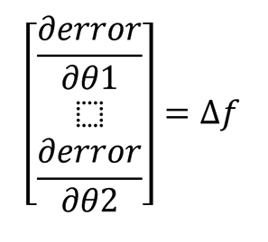
Equation 2: Vector Gradient

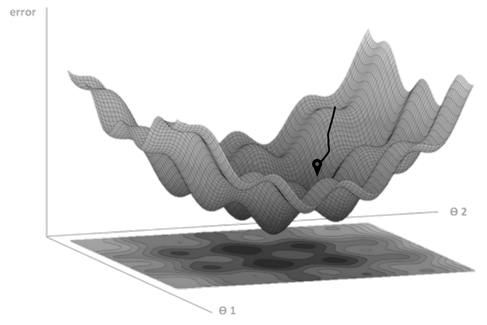
Figure 5: Descent Gradient Graphic.

Source: Adapted from YouTube portal: DotCSV

The system is to be complete when the learning rate (a) is added, which defines how much the gradient affects the updating of our parameters in each iteration or, what is the same, how much progress is made in each step. Equation 3

θ=θ-a*∆f

Equation 3: Weight update

Backpropagation

The “backpropagation” (Werbos, 1994), is perhaps the most used algorithm for ANN training (Wasserman, 1989). The backpropagation algorithm consists of 2 steps: first, each input pattern of the training dataset is passed through the ANN from the input layer to the output layer. The network output is compared to the desired target output (observed data) and an error based on the cost function is calculated. The second step is when the error propagates backward through the ANN at each node (neuron) and the connection weights are adjusted accordingly.

Cost Function

The cost function is responsible for quantifying the distance between the real and predictive values by the ANN. In other words, it measures how much the network is wrong when making predictions. In most cases, the cost function returns positive values. The closer the cost value is to zero, the better the network predictions (less error). In this case, since it is a regression problem, the root mean square error or RMSE function is used. Equation 4

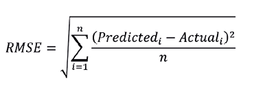
Equation 4: Cost Function: RMSE

Validation Model

Similar to hydrological and hydrogeological modeling, the performance of a trained ANN can be evaluated by subjecting it to new patterns that it has not seen during training. This performance is estimated from a cost function that relates the predicted and observed data. During preprocessing, the dataset was divided into training data and test data, the latter being vital for validation. With the adjusted ANN model, its performance is measured by entering the test data (Figure 4) and evaluating the generated or predictive data versus the test data using equation 4 and finally obtaining the best model.

2.4. Algorithms and packages

For the treatment of data, graphs, and calculations, different libraries of the Python programming language have been used. The benefits of using this language are: it is open source, a simple language with great potential, it includes a very wide community of collaborators, and growth in the projection of new libraries to be applied, among others. The libraries used in this study were:

NumPy which provides support for creating large multidimensional arrays and vectors, along with a large collection of high-level mathematical functions to operate on them, (Oliphant, 2005). Pandas is a library of software, which offers data structures and operations to manipulate numerical tables and time series. (McKinney, 2008).

Matplotlib is a library for generating plots from data contained in lists or arrays (D. Hunter, 2003). Scikit-learn or better known as Sklearn is a machine learning (ML) library. It includes various classification, regression, and group analysis algorithms, among which are support vector machines, random forests, and K-means, among others (Pedregosa et al, 2010).

3. Results and recommendations

3.1. ANN model characteristics

The organization and structuring of the input data and the identification of the most appropriate parameters are the most complex activities in the development of ANN models. This section presents the results of the parameters and mean square error of the cross-validations.

With the hyperparameters, the ANN performed well at the architectural level (1 hidden layer with 10 neurons). Additionally, the learning rate value was configured in such a way that it adopted values of 10-2 and 10-1, which in the end the model opted for the value of 10-2 since a lower value implies that the optimization process does not go jumping regions to another and achieving convergence for the established iteration number. Finally, regarding the alpha parameter, it initially presented 10 values that range between 10-3 and 103, but the regressor model after the iterations learned with the value of 0.0215, that is, 10-1.666.

With the adjusted parameters, the regressor model provided an RMSE of 0.05, which is acceptable because it is less than 0.8, using the solver =’lbfgs’ configuration, which allows optimizing the values, converging faster and performing better. Figure 6 shows the architectural configuration of the ANN. Each input is multiplied by a weight (synaptic arrow) and then within the neuron the weighted sum of xi*wi + b*w is performed, which is evaluated in the activation function (ReLU) and the result is the y value within a neuron for the hidden layer. This process is repeated until the value is obtained in the output neuron.

3.2. Results

After evaluating the efficiency of the ANN model to estimate Gr, the results of the ANN for the different soil textures in the study area are presented. In this case, each texture (S01, S02, S03) has the same number of predictors and observations on the same time scale (2005-2020), varying the physical properties of the soil, and this implies different observation values of the variables.

The results indicate, under the same initial configurations in each ANN, a fit is obtained according to the parameters, being evaluated with RMSE < 0.8, thus concluding that the models are acceptable. Within the adjustment or learning process, it is observed that for the same architecture and iteration number, the ANNs opted for the lowest value of learning rate, this being the best optimizer for the prompt convergence and solution of the model; however, each RNA opted for a different alpha value, but within the ranges of 10-3 and 103. Table 1

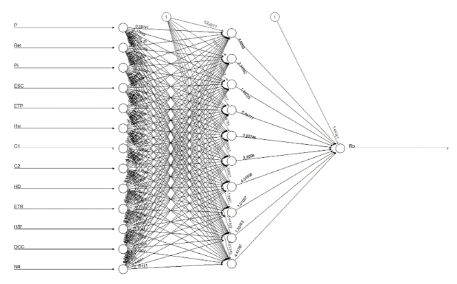
Figure 6: ANN architectural configuration for S01. Source: self-made

Table 1: ANN configuration for soil textures. Source: self-made

The results of the study have identified the relationship between each of the variables and parameters with which the regressor model was designed, configured, and adjusted. Based on the estimation of errors, the prediction model is acceptable concerning the conceptual model. This implies that a nonlinear regressor model of the RNA type is capable of making estimates and predictions of hydrogeological variables.

3.3. Recommendations

For future work, the design and development of a set of programs are recommended to collect and integrate observations of more variables in time and space, in such a way that a database is generated that makes it possible to use these in a simple and interoperable way. ANN models work better when the information of different variables related to the phenomenon in question is longer and more complete.

Design a hydrogeological database capable of storing information in a “silo” and that its design is ‘relational’ or ‘non-relational’ depending on the variability, volume, and speed with which these data are produced.

The development of new research using RNA with data on precipitation, temperature, and groundwater level in unconfined aquifers is recommended. This is because the changes in groundwater levels (descent and ascent) are related to the dry and wet periods.

4. Acknowledgments

To INETER, UNAN- Managua, and FAO because the Project: “Improvement of hydrometeorological and climatic information systems to favor investments in climate change in Nicaragua”, provided the opportunity to develop this research in the field of Geoinformatics and Hydroinformatics, to contribute to the professional development of specialists in hydrology in Nicaragua and Central America.